Runs locally on my i7 with NVidia 3050.

TOC

1 Output
2 PY script
3 Training/inference summary
4 Code with detailed comments. Great commentary for each line of the code (from GPT). Study this closely to understand the gist of this core first demo.

For details see #607_2.1_predictive_NNs_.docx.

1 Output

device: cuda
epoch=0 loss=0.505204
epoch=100 loss=0.000351
epoch=200 loss=0.000070
epoch=300 loss=0.000034
epoch=400 loss=0.000024
epoch=500 loss=0.000018
epoch=600 loss=0.000015
epoch=700 loss=0.000012
epoch=800 loss=0.000010
epoch=900 loss=0.000008

drones

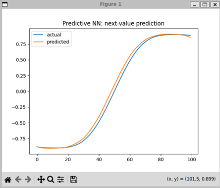
2 PY script

# pred_nn_01_sine.py
# Predictive NN demo:
# current/recent state -> future state

import math
import torch
import torch.nn as nn
import matplotlib.pyplot as plt

# -----------------------------
# 1 device
# -----------------------------

device = "cuda" if torch.cuda.is_available() else "cpu"
print("device:", device)

# -----------------------------
# 2 create synthetic data
# -----------------------------

N = 2000
window = 20

t = torch.linspace(0, 80, N)
series = torch.sin(t) + 0.1 * torch.sin(3 * t)

X = []
Y = []

for i in range(N - window - 1):
    X.append(series[i:i + window])
    Y.append(series[i + window])

X = torch.stack(X).to(device)
Y = torch.stack(Y).unsqueeze(1).to(device)

# -----------------------------
# 3 small predictive NN
# -----------------------------

model = nn.Sequential(
    nn.Linear(window, 64),
    nn.ReLU(),
    nn.Linear(64, 64),
    nn.ReLU(),
    nn.Linear(64, 1),
).to(device)

loss_fn = nn.MSELoss()
optimizer = torch.optim.Adam(model.parameters(), lr=0.001)

# -----------------------------
# 4 train
# -----------------------------

for epoch in range(1000):
    pred = model(X)
    loss = loss_fn(pred, Y)

    optimizer.zero_grad()
    loss.backward()
    optimizer.step()

    if epoch % 100 == 0:
        print(f"epoch={epoch} loss={loss.item():.6f}")

# -----------------------------
# 5 predict next values
# -----------------------------

model.eval()

start = 1500
input_window = series[start:start + window].clone().to(device)

predicted = []

with torch.no_grad():
    for _ in range(100):
        y = model(input_window.unsqueeze(0))
        predicted.append(y.item())

        input_window = torch.cat([
            input_window[1:],
            # y.squeeze()
            y.reshape(1)
        ])

actual = series[start + window:start + window + 100].cpu()

# -----------------------------
# 6 plot
# -----------------------------

plt.plot(actual.numpy(), label="actual")
plt.plot(predicted, label="predicted")
plt.legend()
plt.title("Predictive NN: next-value prediction")
plt.show()

3 Training/inference summary

TRAINING PHASE

Generate signal

t ───────────────────────────────►

series =
sin(t)
+
0.1*sin(3t)

Result:
smooth wave + small wiggles

Create training windows

[x0 x1 x2 x3 x4] ──► x5
[x1 x2 x3 x4 x5] ──► x6
[x2 x3 x4 x5 x6] ──► x7

Tensor shapes

X : [samples, window]
Y : [samples, 1]

Neural network

Input window
[ x(t-20) ... x(t-1) ]
            │
            ▼

Linear(20 → 64)
            │
            ▼
ReLU
            │
            ▼

Linear(64 → 64)
            │
            ▼
ReLU
            │
            ▼

Linear(64 → 1)
            │
            ▼

Predicted next value
x(t)

Training loop

Forward pass:
X ─► model ─► prediction

Loss:
prediction vs actual

MSE:
(pred - actual)^2

Backprop:
loss.backward()

Optimizer:
Adam updates weights

Repeat 1000 epochs

GENERATION / INFERENCE PHASE

Initial known window

[x1500 ... x1519]

            │
            ▼

model predicts:

x1520

append prediction

old:
[x1500 ... x1519]

new:
[x1501 ... x1520]

Repeat autoregressively

[x1501 ... x1520] ─► x1521
[x1502 ... x1521] ─► x1522
[x1503 ... x1522] ─► x1523

Core autoregressive loop

past values
    │
    ▼
predict next value
    │
    ▼
feed prediction back in
    │
    ▼
repeat

Comparison

predicted future
vs
actual future

Important conceptual connection

This is structurally similar to LLM generation:

previous tokens
    │
    ▼
predict next token
    │
    ▼
append token
    │
    ▼
repeat

4 Code with detailed comments

2 create synthetic data

N = 2000
window = 20
t = torch.linspace(0, 80, N)
series = torch.sin(t) + 0.1 * torch.sin(3 * t)
X = []
Y = []
for i in range(N - window - 1):
    X.append(series[i:i + window])
    Y.append(series[i + window])

So the NN learns:
past values  ->  predict next value
Example:
If:
window = 5
and the series is:
[10, 11, 12, 13, 14, 15, 16]
then one training sample becomes:
X = [10,11,12,13,14]
Y = 15
next sample:
X = [11,12,13,14,15]
Y = 16
So the code is building many examples like:
[past sequence] -> next number
ASCII visualization:
t0 t1 t2 t3 t4 -> t5
t1 t2 t3 t4 t5 -> t6
t2 t3 t4 t5 t6 -> t7
This is fundamentally sequence prediction.
The NN is learning:
f(x_(t-window),...,x_(t-1))≈x_t
Very important concept:
the network is NOT learning “time”.
It only learns numerical relationships between patterns inside the window and the next output.

X = torch.stack(X).to(device)

Before this:
X = [tensor(...), tensor(...), tensor(...)]
a Python list of many tensors.
torch.stack(X) combines them into one big tensor.
Shape becomes something like:
[number_of_samples, window]
Example:
[1000, 20]
meaning:
1000 training examples
20 numbers per example
Then:
.to(device)
moves the tensor to GPU memory because:
device = cuda

Y = torch.stack(Y).unsqueeze(1).to(device)

Same idea, but:
.unsqueeze(1)
adds an extra dimension.
Without unsqueeze:
[1000]
With unsqueeze:
[1000,1]
ASCII:
before:
[ y1 y2 y3 y4 ]
after:
[
 [y1]
 [y2]
 [y3]
 [y4]
]
This is needed because the NN output layer likely produces:
batch_size x 1
So target and prediction shapes must match.
Typical flow:
X:
[batch, window]
↓
NN
↓
prediction:
[batch, 1]
↓
compare with Y:
[batch, 1]
This is one of the most important PyTorch concepts:
tensor shape management
Most beginner bugs in PyTorch are actually shape bugs.

3 small predictive NN

model = nn.Sequential(
    nn.Linear(window, 64),
    nn.ReLU(),
    nn.Linear(64, 64),
    nn.ReLU(),
    nn.Linear(64, 1),
).to(device)

input(window values)
        ↓
Linear(window → 64)  // basic detectors
        ↓
ReLU
        ↓
Linear(64 → 64)     // combinations of detectors
        ↓
ReLU
        ↓
Linear(64 → 1)    // Produces one number: predicted next value
        ↓
predicted next value
So the network implements approximately:
f(x_(t-window),...,x_(t-1))≈x_t
This network has NO explicit sine equation.
It never sees:
sin(x)
It only sees examples:
past numbers → next number
and learns an approximation function through weight adjustment.

loss_fn = nn.MSELoss()

loss_fn = nn.MSELoss()
MSE = Mean Squared Error.
Formula:
MSE=1/N ∑_(i=1)^N▒( y_i-y ̂_i )^2
Mechanistically:
prediction - actual
↓
square it
↓
average all errors
Example:
actual     = 0.80
prediction = 0.70
error:
0.80 - 0.70 = 0.10
squared:
0.10² = 0.01
Why square?
1. removes negative signs
2. large errors become much larger
Example:
0.1² = 0.01
1.0² = 1.00
So large mistakes are punished heavily.

optimizer = torch.optim.Adam(model.parameters(), lr=0.001)

optimizer = torch.optim.Adam(model.parameters(), lr=0.001)
Adam updates all weights and biases.
Conceptually:
1. compute loss
2. compute gradients
3. adjust weights slightly
4. repeat thousands of times
Very rough update idea:
W_new=W-η ∂L/∂W
where:
W  = weight
L  = loss
η  = learning rate
learning rate
lr=0.001
controls step size.
Too large:
weights jump wildly
training unstable
Too small:
training extremely slow

4 train

for epoch in range(1000):
    pred = model(X)
Runs the neural network.
Mechanistically:

X
↓
Linear
↓
ReLU
↓
Linear
↓
ReLU
↓
Linear
↓
prediction
Produces:
pred
which is the predicted next value for every training sample.

    loss = loss_fn(pred, Y)

Compares:
prediction
vs
actual answer
using MSE.
Result:
- single scalar error value
Example:
- loss = 0.527
large error early in training.
Later:
- loss = 0.000018
very accurate predictions.

    optimizer.zero_grad()

PyTorch accumulates gradients by default.
So before new backprop:
old gradients must be cleared

    loss.backward()

This is the big one.
PyTorch computes:
how much every weight contributed to error
Mathematically:
∂L/∂W
for ALL weights.
Meaning:
if this weight increases slightly,
does loss go up or down?
This uses the chain rule through all layers.
ASCII idea:
loss
 ↑
output layer
 ↑
hidden layer
 ↑
hidden layer
 ↑
input
Error information flows backward through the network.
Hence:
backpropagation

    optimizer.step()

Adam now updates weights using gradients.
Conceptually:
bad weights → adjusted
good weights → reinforced
Repeated many times:
network slowly learns function approximation

    if epoch % 100 == 0:
        print(f"epoch={epoch} loss={loss.item():.6f}")

prints every 100 epochs.
Your output:
epoch=0   loss=0.527
epoch=900 loss=0.000018
shows successful convergence.

5 predict next values

model.eval()

This switches the network into:
inference mode
meaning:
training is finished
now only do prediction
You currently only have:
Linear
ReLU
So:
model.eval()
does not visibly change behavior much.
But it is still correct practice.
Typical workflow:
model.train()
    training mode
model.eval()
    inference mode
Conceptually:
train mode:
learn weights
eval mode:
freeze behavior and predict
Very important in larger real-world models.

start = 1500
input_window = series[start:start + window].clone().to(device)

This selects the initial sequence used for prediction.
Mechanistically:
start = 1500
chooses a position inside the sine series.
Then:
series[start:start + window]
extracts a chunk of past values.
If:
window = 20
then this becomes:
series[1500:1520]
ASCII:
t1500 t1501 t1502 ... t1519
These are the known past values.
clone()
.clone()
creates a copy.
Without clone:
input_window may share memory
with original tensor
Clone gives an independent tensor.
to(device)
.to(device)
moves the tensor to GPU:
cuda
so model and data are on same device.
Final meaning
input_window
contains the recent history used to predict the future.
Conceptually:
past sequence
→
predict next value
The network now does autoregressive prediction:
predict one value
append it
predict next value
append it
repeat
Very similar to how LLMs generate tokens:
previous tokens
→ predict next token
→ append
→ repeat
This is an extremely important connection.
Your sine predictor is structurally similar to transformer generation loops:
x_(t-window:t-1)→x_t

(code below)

This is the autoregressive prediction loop.
This is the MOST important part conceptually.
ASCII overview:
initial window
      ↓
predict next value
      ↓
append prediction
      ↓
shift window
      ↓
predict again
      ↓
repeat
This is fundamentally similar to LLM token generation.

predicted = []
with torch.no_grad():

no_grad():
disables gradient computation.
Because:
we are no longer training
Benefits:
- less memory
- faster
- no backprop graph

    for _ in range(100):

generate 100 future values.

        y = model(input_window.unsqueeze(0))

input_window.unsqueeze(0)
adds batch dimension.
Without:
[window]
With:
[1, window]
because Linear layers expect batches.
ASCII:
single sample:
[20]
batch of 1:
[1,20]
run model
y = model(...)
predicts the next value.
Conceptually:
x_(t-window:t-1)→x_t

        predicted.append(y.item())

.item() converts: 
tensor → Python number

        input_window = torch.cat([
            input_window[1:],
            y.squeeze()
        ])

sliding window update
This is the key mechanism.
input_window[1:]
drops oldest value.
ASCII:
before:
[a b c d e]
after:
[b c d e]
Then:
y.squeeze()
removes extra dimensions from prediction.
Then:
torch.cat([...])
appends new prediction.
Result:
old window:
[a b c d e]
predicted:
[f]
new window:
[b c d e f]

actual = series[start + window:start + window + 100].cpu()

This line extracts the:
- actual future values
from the original sine series.
Mechanistically:
actual = series[start + window : start + window + 100]
means:
start after the input window
then take next 100 real values
Example.
If:	
start = 1500
window = 20
then:
series[1520:1620]
is extracted.
ASCII:
known input window:
[1500 ........ 1519]
actual future:
[1520 ........ 1619]
So:
actual
contains the TRUE future values.
Meanwhile:
predicted
contains the NN-generated future values.
Then the graph compares:
predicted vs actual
And:
.cpu()
moves the tensor from GPU memory back to CPU memory.
Needed because plotting libraries usually expect CPU tensors.

Extremely important concept

After first prediction:
the model starts consuming its OWN outputs
not real training data anymore.
This is true autoregressive generation.
Same core idea as LLMs:
previous generated tokens
→ predict next token
→ append
→ repeat
Important limitation
Errors accumulate.
Small mistakes become future input.
So over long generation:
prediction drift occurs
Exactly like hallucination drift in LLMs.
Very deep conceptual connection:
sequence predictor
=
autoregressive generator
Your sine-wave NN is a tiny version of the same generation principle used by transformers.

6 plot

plt.plot(actual.numpy(), label="actual")
plt.plot(predicted, label="predicted")
plt.legend()
plt.title("Predictive NN: next-value prediction")
plt.show()

26.0525