Runs locally on my i7 with NVidia 3050.

drones

TOC

1 Output
2 PY script
3 Training/inference summary
4 Code with detailed comments. Great commentary for each line of the code (from GPT). Study this closely to understand the gist.
3.1.1 Tiny NN demo (D2ccc) INFERENCE / TRAINING

For details see #607_2.1_core_NNs_.docx.

1 Output

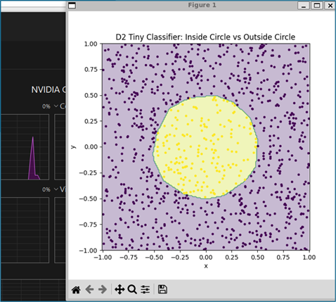
device: cuda
epoch=0 loss=0.753134 accuracy=0.1790
epoch=100 loss=0.136629 accuracy=0.9640
epoch=200 loss=0.055828 accuracy=0.9940
epoch=300 loss=0.030925 accuracy=0.9970
epoch=400 loss=0.019975 accuracy=0.9990
epoch=500 loss=0.013983 accuracy=1.0000
epoch=600 loss=0.010112 accuracy=1.0000
epoch=700 loss=0.007658 accuracy=1.0000
epoch=800 loss=0.005994 accuracy=1.0000
epoch=900 loss=0.004811 accuracy=1.0000

drones

2 PY script

# d2_tiny_classifier.py

import torch
import torch.nn as nn
import matplotlib.pyplot as plt

# -----------------------------
# D2 Tiny Classification Demo
# -----------------------------

device = "cuda" if torch.cuda.is_available() else "cpu"
print("device:", device)

# 1. Create fake 2D data
N = 1000

# random x,y points between -1 and +1
X = torch.rand(N, 2) * 2 - 1

# class rule:
# if point is inside circle -> class 1
# otherwise -> class 0
radius = torch.sqrt(X[:, 0] ** 2 + X[:, 1] ** 2)
Y = (radius < 0.5).long()

X = X.to(device)
Y = Y.to(device)

# 2. Define classifier
model = nn.Sequential(
    nn.Linear(2, 16),
    nn.ReLU(),
    nn.Linear(16, 16),
    nn.ReLU(),
    nn.Linear(16, 2),  # 2 class scores/logits
).to(device)

# 3. Loss + optimizer
loss_fn = nn.CrossEntropyLoss()
optimizer = torch.optim.Adam(model.parameters(), lr=0.01)

# 4. Train
for epoch in range(1000):
    logits = model(X)
    loss = loss_fn(logits, Y)

    optimizer.zero_grad()
    loss.backward()
    optimizer.step()

    if epoch % 100 == 0:
        pred_class = logits.argmax(dim=1)
        accuracy = (pred_class == Y).float().mean()
        print(
            f"epoch={epoch} "
            f"loss={loss.item():.6f} "
            f"accuracy={accuracy.item():.4f}"
        )

# 5. Plot decision boundary
model.eval()

grid_size = 200
xx, yy = torch.meshgrid(
    torch.linspace(-1, 1, grid_size),
    torch.linspace(-1, 1, grid_size),
    indexing="ij",
)

grid = torch.stack([xx.reshape(-1), yy.reshape(-1)], dim=1).to(device)

with torch.no_grad():
    grid_logits = model(grid)
    grid_pred = grid_logits.argmax(dim=1).cpu()

Z = grid_pred.reshape(grid_size, grid_size)

plt.figure(figsize=(6, 6))
plt.contourf(xx, yy, Z, alpha=0.3)

plt.scatter(
    X[:, 0].cpu(),
    X[:, 1].cpu(),
    c=Y.cpu(),
    s=8,
)

plt.title("D2 Tiny Classifier: Inside Circle vs Outside Circle")
plt.xlabel("x")
plt.ylabel("y")
plt.axis("equal")
plt.show()

3 Training/inference summary

TRAINING PHASE

xxxxx

GENERATION / INFERENCE PHASE

xxxx

4 Code with detailed comments

xxx

output

Extremely important concept

text2

3.1.1 Tiny NN demo (D2ccc) INFERENCE (see section 5 at the end of this page for code description)

“Inference” means normal run-time operation. Generating output from input. Training is described next.

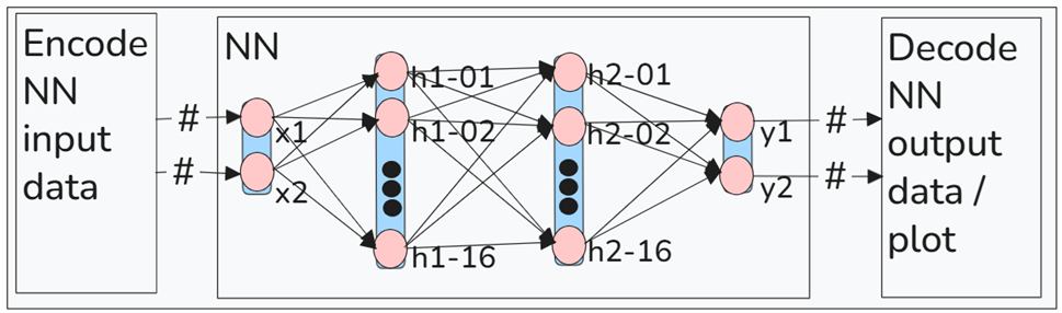
This one simple NN demo will give you an understanding of the core of all AI (including CNNs, LLMs TFs, etc). The following diagram shows the core components of the demo:

Encoder. All NNs only “know” numbers (including ChatGPT, Claude, etc). So if you have a dataset that is not (FP) numbers, it must be encoded (and later decoded).
NN. The source of “intelligence”. A UFA (universal function approximator).
- This NN inputs 2 numbers. And based on that number outputs 2 probabilities. That’s it.
- It does this using the “neurons” shown. Rather than using a logical mathematical equation for distance from center, D2ccc’s “neurons” calculate the equation W*x+b for all the lines shown (see section 5 for details). This is absolutely deterministic and without one iota of intelligence”.
- NOTE: This is very confusing, but typical in AI discussions. In the NN diagram “x1” and “x2” are in the plot “x” and “y”. NN diagram output “y1” and “y2” are the probabilities that the point is in the center green circle or not.
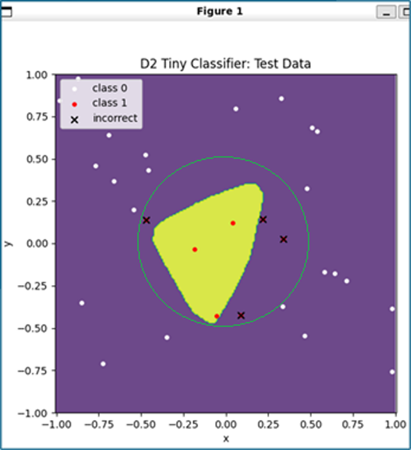
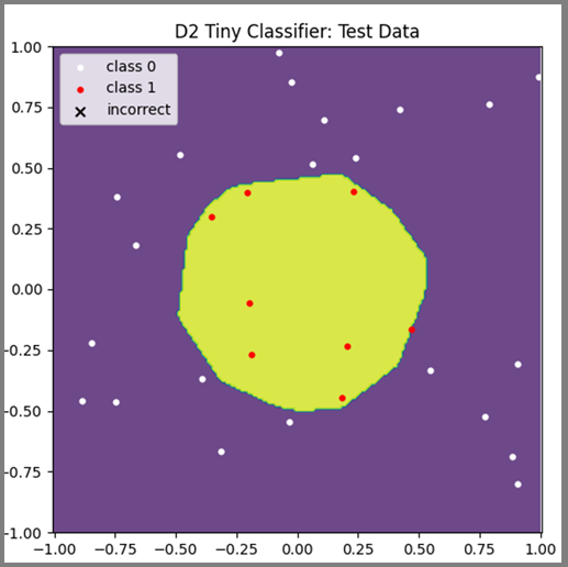
- The yellow area is the center of the circle as programmed into the NN by the training data. I intentionally lowered the training data so that the approximation error would be visible.
- White dots are not in the center. Red dots are in the center. These are calculated by the NN.
- The black X’s show data points that the NN mistakenly classified as outside the circle.
- The genius of the NN is that it can take a data combination that it has never seen and still make a good guess as to what the data is. That is also the NN’s weakness.
- This is why scaling is so important. Because AI has no intelligence. But with much more brute force calculation, the error rate of the UFA can go down enough to give the illusion of intelligence. The marketing/hype genius of Musk is that can make “batteries” in a car a status symbol, and make “macrohard” (brute force computing) a status symbol for AI.
- REMEMBER: The NN knows nothing about x,y, the circle, etc. It only computes numbers. And the NN is a clocked binary state machine. Intelligence (human style) exists in time only, not as a series of binary states.
Decoder. Convert from a probability for inside/outside the circle to a binary state (1 or 0; inside/outside circle).

All of the above insight (and much more) about the CORE of AI from one tiny demo.

Demo D2ccc (left) and test results right)
drones drones

3.1.1b Tiny NN demo (D2ccc) TRAINING

WIP. The main thing is the training input/output must match exactly what is desired in inference. Discuss following steps.

for epoch in range(100):
    logits = model(X)
    loss = loss_fn(logits, Y)
    optimizer.zero_grad()
    loss.backward()
    optimizer.step()

5 NN demo D2cc details

Note: I created this version of the D2 demo on 26.0611. I documented the details in docx #607. Its similar to D2 demo on page 2.1 Core NNs.

1) The short bit of code shown below defines the D2ccc Tiny Demo classifier NN.

model = nn.Sequential(
    nn.Linear(2, 16),
    nn.ReLU(),
    nn.Linear(16, 16),
    nn.ReLU(),
    nn.Linear(16, 2),  # 2 class scores/logits
).to(device)

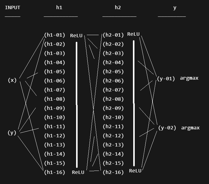
2) This is the resulting NN.

- W = weights, b = biases (these are the model parameters that are UPDATED during training and FIXED during inference)
- h1-01 = hidden layer 1, neuron 01
- h1-02 = hidden layer 1, neuron 02
- ...
- h2-1 = hidden layer 2, neuron 01
- ...
- y-1  = output neuron 1
- y-2  = output neuron 2

50 data points
100 epochs
num_test = 30

drones

3) Computation details.

x, y (inputs)
        ▼
Layer 1: nn.Linear(2,16)
 h1_1 = w1*x + w2*y + b  → ReLU → a1_1
 ...
 h1_16= w1*x + w2*y + b  → ReLU → a1_16
        ▼
Layer 2: nn.Linear(16,16)
 h2_1 = w1*a1_1 + w2*a1_2 + ... + w16*a1_16 + b  → ReLU → a2_1
 ...
 h2_16= w1*a1_1 + w2*a1_2 + ... + w16*a1_16 + b  → ReLU → a2_16
       ▼
Output layer: nn.Linear(16,2)
 logit_outside = w1*a2_1 + w2*a2_2 + ... + w16*a2_16 + b
 logit_inside  = w1*a2_1 + w2*a2_2 + ... + w16*a2_16 + b
        ▼
argmax(logits)
        ▼
class 0 = outside circle
class 1 = inside circle

4) These are the total number of computations within the NN.

TOTALS
- 354 wx+b operations + 32 ReLU operations = 386 simple operations per point
- weights: 32 + 256 + 32 = 320
- biases: 16 + 16 + 2 = 34
- total parameters = 354
- ReLU after h1: 16 comparisons
- ReLU after h2: 16 comparisons

5) Resulting output (I will explain these results better later).

I intentionally lowered the training length to make the result less than optimal (easier to see).
I added the green circle. It shows where the boundary should be (in this demo you could compute the test points to see if they were in the center; an equation would work; but the point of this demo is to show how to can do that without equations and what results would be; this would be valuable for data sets that cannot be classified by a simple equation).
Yellow / purple area boundary was the NN-computed from a limited data set.
White dots = outside area.
Red dots = NN corrected classified as in the green circle.
X marks = NN incorrectly classified as outside the green circle.

test 1

50 data points
100 epochs
num_test = 30

drones

test 2

500 data points
1000 epochs
num_test = 30

drones

6) Lessons learned from this demo:

The simple NN can classify x,y locations with good accuracy.
But classification accuracy is not equation-level perfect. In our simple demo the results were good for a small NN. But for more complex datasets the size of the NN would increase dramatically. AI must be used where the input / output relationship can not be defined with simple computation or equations. But AI is always an approximation (UFA, universal function approximator), so the challenge is integrating AI so that the approximation errors are acceptable (for war time planning systems OK, for self driving cars or home humanoids NOT OK).

26.0616 (0526)