D8.6 Inference app (2c)
See the working text for this QS in
- #619_.docx.
- Demo URL there are actually many … this was a chaotic demo.
TOC
- 6.0 overview
- 6.1 ME: how can i test this model? using pipeline, or just some simple verification test
- 6.2 ME: pipeline test step by step (BINGO BINGO)
- 6.3 Deploy the model (done already in 2b in Jupyter notebook)
- 6.4 Publish the model as a Function
- 6.5 Create a Workshop app (UI) (BINGO)
6 (AIP/FDE) interactive inference app 26.0721-22
6.0 overview
Goal:
Let a user enter feature values in a Workshop UI and get a live model prediction.
- fUser inputs → Function → Live model deployment → Prediction displayed in Workshop
your next logical demo can be:
Build a tiny Workshop app that lets me type three numbers and returns a model prediction.
Important distinction
| Use case | Tool |
|---|---|
| Predict many rows and save dataset | Pipeline Builder batch inference |
| Let user enter values and get one prediction | Workshop + Function + live model |
| Compare predictions to actual values | Dataset / pipeline / notebook |
| Operational app for users | Workshop |

What you have now: batch inference
Current flow:
dataset rows → model → prediction dataset
This is good for predicting many rows at once.
What you want next: interactive inference app
Desired flow:
user enters values in UI ↓
model runs once ↓
prediction shown on screen
Example user inputs:
median_income = 5.2
housing_median_age = 30
total_rooms = 3000
Output:
predicted median house value = 256,000
Simplest Palantir architecture
Workshop app ↓
Input widgets / variables ↓
Function or published model function ↓
Live model deployment ↓
Display prediction
6.1 ME: how can i test this model? using pipeline, or just some simple verification test
(was 2b.6)
(1) You can test it simply in the notebook first. That is the easiest verification.
Simple notebook test
Run this in a new cell:
X_test = test_df[numeric_features]
y_test = test_df[“median_house_value”]
predictions = model.predict(X_test)
predictions[:10]
array([256476.21159013, 337128.08977048, 497948.74113868, 236398.49173821,
204920.20851306, 258905.02382699, 283067.71580942, 158815.6017816 ,
699570.17961624, 182801.35751066])
That should show the first 10 predicted house values.
Compare predictions to actual values
Run:
import pandas as pd
results = test_df.copy()
results[“predicted_median_house_value”] = predictions
results[“error”] = results[“predicted_median_house_value”] - results[“median_house_value”]
results[
[
“median_income”,
“housing_median_age”,
“total_rooms”,
“median_house_value”,
“predicted_median_house_value”,
“error”,
]
].head(10)
This gives you a simple visual check:
actual value vs predicted value
| median_income | housing_median_age | total_rooms | median_house_value | predicted_median_house_value | error | |
|---|---|---|---|---|---|---|
| 2 | 4.8984 | 31.0 | 3073.0 | 311700.0 | 256476.211590 | -55223.78841 |
| 3 | 6.4958 | 37.0 | 3333.0 | 500001.0 | 337128.089770 | -162872.91023 |
| 5 | 10.6796 | 28.0 | 3539.0 | 500001.0 | 497948.741139 | -2052.258861 |
| 17 | 4.252 | 31.0 | 4949.0 | 436700.0 | 236398.491738 | -200301.508262 |
| 18 | 3.6769 | 31.0 | 3155.0 | 450000.0 | 204920.208513 | -245079.791487 |
| 27 | 5.9263 | 3.0 | 6577.0 | 251800.0 | 258905.023827 | 7105.023827 |
| 28 | 5.5061 | 17.0 | 10267.0 | 239400.0 | 283067.715809 | 43667.715809 |
| 37 | 2.2304 | 42.0 | 1558.0 | 203800.0 | 158815.601782 | -44984.398218 |
| 40 | 15.0001 | 36.0 | 4152.0 | 500001.0 | 699570.179616 | 199569.179616 |
| 46 | 2.9934 | 35.0 | 2914.0 | 350000.0 | 182801.357511 | -167198.642489 |
Calculate basic error metric
Run:
from sklearn.metrics import mean_absolute_error, r2_score
mae = mean_absolute_error(y_test, predictions)
r2 = r2_score(y_test, predictions)
mae, r2
(59094.622737489306, 0.5194416988275954)
Interpretation:
MAE = average prediction error in dollars.
R² = how much variation the model explains.
closer to 1.0 is better,
around 0 means weak,
negative means bad.
Quick single-row test
sample = X_test.head(1)
model.predict(sample)
array([256476.21159013])
Do you need a pipeline? Not yet.
Use:
Notebook test first
Then later:
batch inference pipeline
if you want to apply the model to a full dataset and write predictions to Foundry.
Minimal verification
Run this:
X_test = test_df[numeric_features]
y_test = test_df[“median_house_value”]
predictions = model.predict(X_test)
from sklearn.metrics import mean_absolute_error, r2_score
print(“MAE:”, mean_absolute_error(y_test, predictions))
print(“R2:”, r2_score(y_test, predictions))
print(predictions[:10])
MAE: 59094.622737489306
R2: 0.5194416988275954
[256476.21159013 337128.08977048 497948.74113868 236398.49173821
204920.20851306 258905.02382699 283067.71580942 158815.6017816
699570.17961624 182801.35751066]
6.2 ME: pipeline test step by step (BINGO BINGO)
(was 2b.7)
The simplest pipeline test is:
housing_test_data → apply model → housing_test_predictions
You are testing whether the published model can take a Foundry dataset as input and produce predictions as a new dataset.
Step 0 — Know what you already have
You already have:
Input dataset
housing_test_data
This has actual known values, including:
median_house_value
Published model
linear_regression_model
Your model expects these input columns:
median_income
housing_median_age
total_rooms
Step-by-step pipeline test
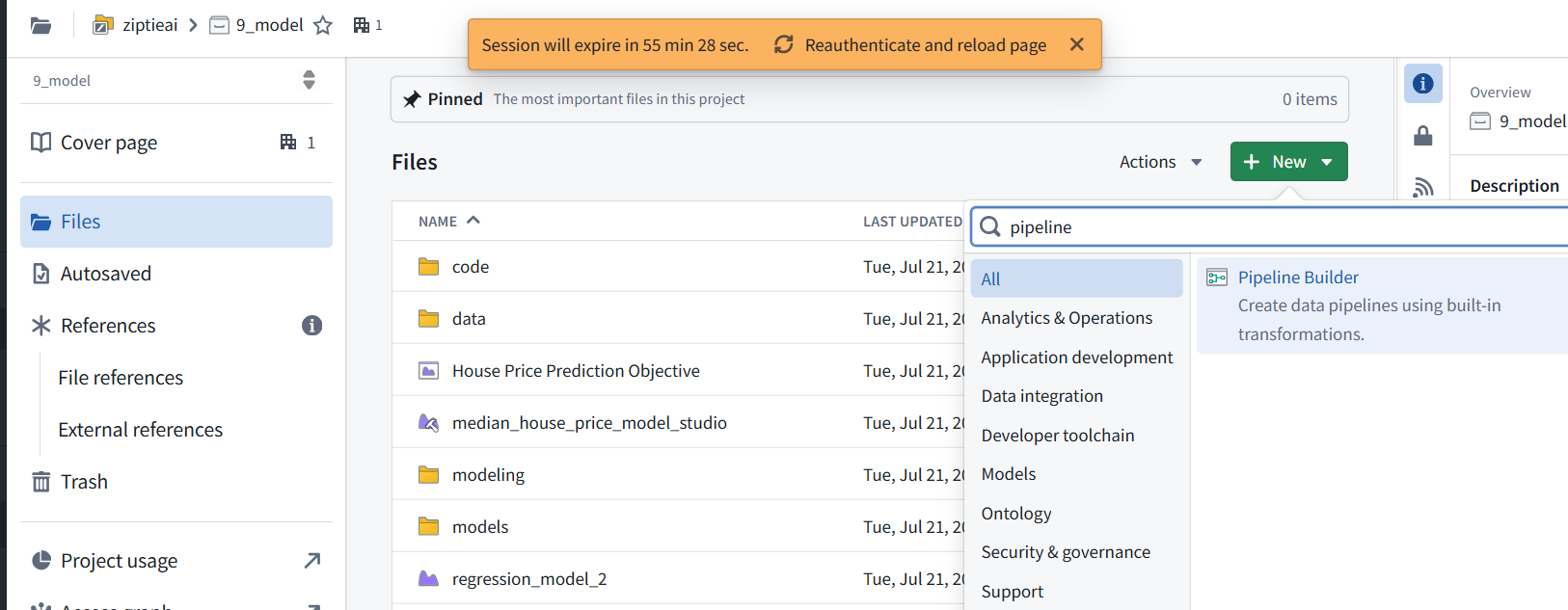
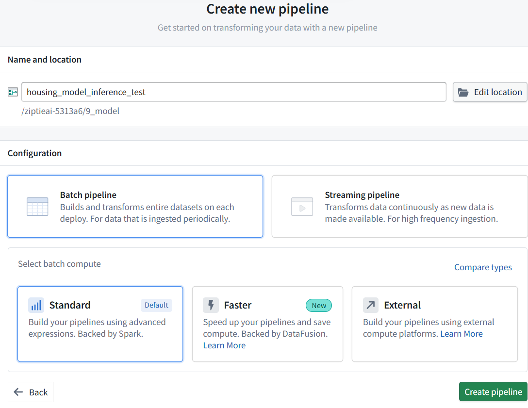
1. Create a new Pipeline Builder pipeline
Go to your project/folder and create a new pipeline.
not 9_model_2
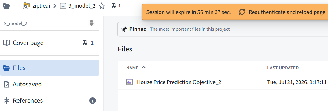
9_model
Name it something simple:
test_model_pipeline
or:
housing_model_inference_test
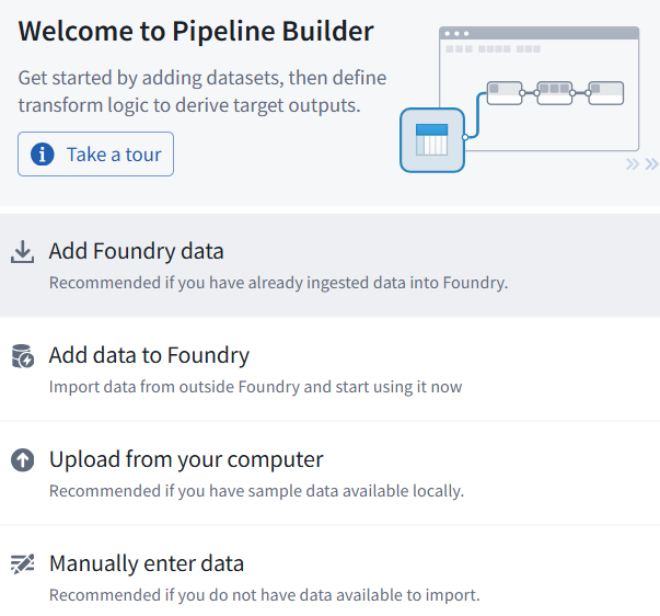
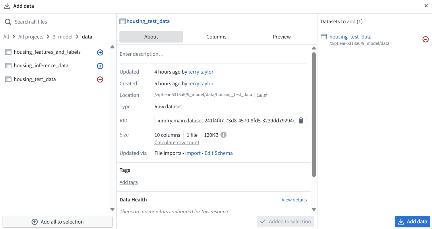
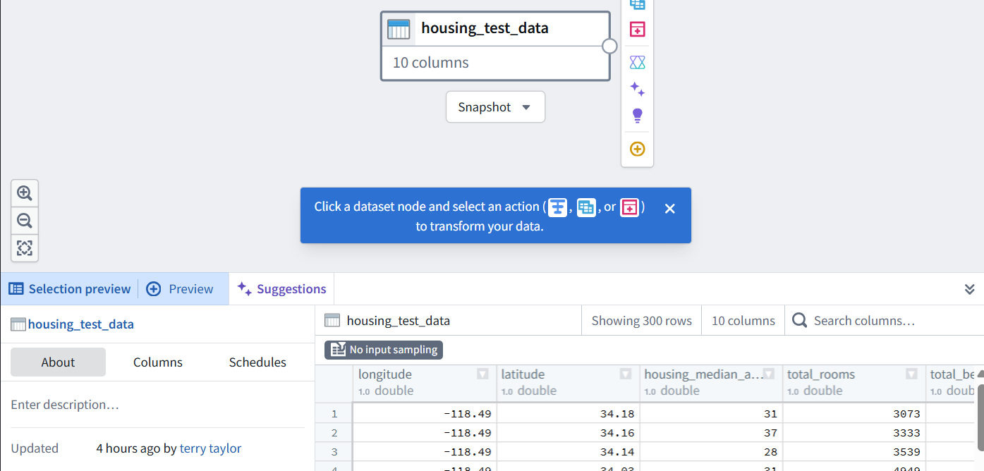
2. Add input dataset
Add dataset:
housing_test_data
This is the dataset you saved from test_df.
26.0903 (v1 26.0903)