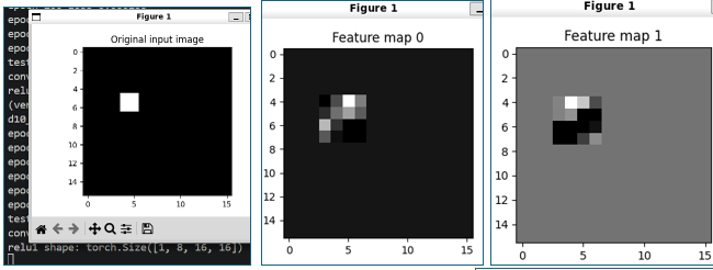
2.2.3 D10 CNN feature map visualization
See also
TOC
- 1 Output
- 2 Code with detailed comments. Great commentary for each line of the code (from GPT). Study this closely to understand the gist.
1 Output
python d9_cnn_defect_detector.py
epoch=0 loss=0.696155
epoch=50 loss=0.020278
epoch=100 loss=0.000759
epoch=150 loss=0.000126
epoch=200 loss=0.000047
epoch=250 loss=0.000026
epoch=300 loss=0.000017
epoch=350 loss=0.000012
epoch=400 loss=0.000009
epoch=450 loss=0.000007
epoch=500 loss=0.000006
labels:
tensor([1., 1., 1., 0., 0., 0.])
predictions:
tensor([1.0000e+00, 1.0000e+00, 9.9999e-01, 6.3785e-06, 6.3786e-06, 6.3786e-06])
(venv) terry@LAPTOP-HKPDHF7M:/mnt/c/Users/terry/Downloads/607_predictive$
2 Code with detailed comments
import torch
import torch.nn as nn
import torch.optim as optim

# ----------------------------
# Generate fake images
# ----------------------------

N = 1000
images = torch.zeros(N, 1, 16, 16)
(batch, channels, height, width)
1000 images, 1 grayscale channel, 16 pixels high, 16 pixels wide
labels = torch.zeros(N, 1)
1000 labels
1 output value each
for i in range(N):
    # defect images
    if i < N // 2:
0-499 defect
500-999 clean
        x = torch.randint(4, 12, (1,)).item()
        y = torch.randint(4, 12, (1,)).item()
random integer
from 4 up to (but not including) 12
create 1 value
Possible results:
tensor([4])
tensor([7])
tensor([11])
.items() extracts the Python value from a 1-element tensor.
Could also write:
  import random
  x = random.randint(4, 11)
Same effect.
The author used PyTorch because the rest of the code is already using tensors.
images[i, 0, y:y+2, x:x+2] = 1.0
image number i
channel 0
rows y through y+1
columns x through x+1
images[5, 0, 10:12, 7:9] = 1.0
which writes:
row 10 col 7 = 1
row 10 col 8 = 1
row 11 col 7 = 1
row 11 col 8 = 1
a 2×2 white square.
labels[i] = 1
this image contains a defect
So the pair becomes:
Image #5  -> has white square -> label 1
Image #700 -> all black       -> label 0
That's the entire supervised-learning dataset:
Input image  --->  Target label
(defect?)         (0 or 1)
The CNN's job is simply to learn:
white square present  -> 1
white square absent   -> 0
# ----------------------------
# CNN
# ----------------------------
model = nn.Sequential(
    nn.Conv2d(1, 8, kernel_size=3, padding=1),
1 input channel, 8 filters, 3x3 detector
Output: [1000, 8, 16, 16]
because padding=1 preserves image size.
    nn.ReLU(),
    nn.Conv2d(8, 16, kernel_size=3, padding=1),
8 feature maps in, 16 feature maps out
Output: [1000, 16, 16, 16]
    nn.ReLU(),
    nn.Flatten(),
This is the important one.
Before:
16 feature maps
16x16 each
Total numbers:
16 × 16 × 16 = 4096
So:
[1000, 16,16,16]
becomes
[1000, 4096]
nn.Linear(16 * 16 * 16, 32),
nn.Linear(4096, 32)
Output:
[1000, 32]
Same idea as your D6 demo.
    nn.ReLU(),
    nn.Linear(32, 1),
Output:
[1000,1]
    nn.Sigmoid()
)
So the whole pipeline is:
[1000,1,16,16]
Conv2d(1→8)
↓ [1000,8,16,16]
Conv2d(8→16)
↓ [1000,16,16,16]
Flatten
↓ [1000,4096]
Linear(4096→32)
↓ [1000,32]
Linear(32→1)
↓ [1000,1]
Sigmoid
↓ probability of defect
loss_fn = nn.BCELoss()
optimizer = optim.Adam(model.parameters(), lr=0.001)

# ----------------------------
# Train
# ----------------------------

for epoch in range(501):
    pred = model(images)
    loss = loss_fn(pred, labels)
    optimizer.zero_grad()
    loss.backward()
    optimizer.step()
    if epoch % 50 == 0:
        print(f"epoch={epoch} loss={loss.item():.6f}")

# ----------------------------
# Test
# ----------------------------

with torch.no_grad():
    test_ids = [0, 1, 2, 500, 501, 502]
image 0,1,2....
p = model(images[test_ids])
creates a new tensor containing only those images.
    print("labels:")
    print(labels[test_ids].squeeze())
    print("predictions:")
    print(p.squeeze())
26.0606 (v1 26.0606)