2.3.6.1b D5 tiny TF algorithm details

← 2.3.6 LLM demos

Work in progress (page created 26.0601).

This a demo that every aspiring AI/ML engineer should study in detail.

This page describes the code for a very basic transformer demo. It describes the python script for

• (1) inference
• (2) training
• (3) NN initialization (of core components)
• (4) NN forward pass (algorithms executed on the components).

This demo runs on a CPU. This demo works with a very small vocabulary consisting of just 7 letters and the space character (in “hello world”). The terms “token” and “letter” are used interchangeably.

See also

• 2.3.6.1 D5 Tiny TF (shows the complete code with no commentary)
• #607_2.1_core_NNs_.docx (lab notes)
• _ziptieai_BOOK2_LLM.docx on the Gdrive

Enter the prompt “h” and the response is “hello world hello world hello world hello “ (letters are generated by TF NN inference)

TOC

• Why study the Tiny Transformer (TF)?
• Core concepts (overview of 4 chapters)
• ch 1 Inference. Enter the letter “h” and the TF returns “hello world hello world hello -world hello”.
• ch 2 Training. Loss and optimizer, training data, and training loop.
• ch 3 NN initialization (init) (create components / define matrices)
• ch 4 NN forward pass (forward()) (use components to execute algorithms)

 

Why study the simple Tiny Transformer?

A short chat with GPT while doing the Tiny Transformer demo. 
ME: This is why I want to do these small demos: Some of these matrix concepts are really difficult at first.
GPT: I think you've discovered something important that many AI courses get wrong. 
Most courses jump immediately to GPT-3 level Attention, Transformers,  LLMs, Agents, etc 
before the student is comfortable with: matrix math, hidden layers, Wx+b, dot products, batches, etc. 
Then people memorize terminology but never develop intuition.

What you've been doing in D5 is closer to how engineers often learn difficult systems:
1. Build the smallest working example.
2. Trace every variable.
3. Understand every matrix shape.
4. Verify every calculation.
5. Scale up later.

For example, working through: Q0K1 = Q0ᵀ·K1 and then connecting it to: scores = Q @ K.transpose(-2,-1) is a big step. 
Many people can recite: attention(Q,K,V) but cannot explain why: 
Q.shape = [8,16], K.shape = [8,16], K.T.shape = [16,8], scores.shape = [8,8].

I also think your instinct about the tiny demos is correct.  
A lot of understanding comes from shrinking the problem. 
GPT-3 has 12288 dimensions, 96 layers, billions of parameters, and is too large to reason about. 
But D5 has 16 dimensions, 1 attention head, 8 tokens, 8-character vocabulary 
and is small enough that you can literally draw every matrix on paper.

The interesting thing is that after a while, the matrix operations stop looking mysterious.
At first: scores = Q @ K.transpose(-2,-1) looks intimidating. 
Then you're starting to see: Compute every Qi·Kj score which is exactly what the code is doing. 
That's the transition from: memorizing AI terminology to understanding the mechanism.

And for someone whose long-term goal is 
agentic AI systems, local LLM stacks, PAL-style systems, and AI platform architecture, that foundation is useful. 
You don't need to become a research mathematician, but being able to look at a transformer
and say "I know what every major matrix multiplication is doing" is a valuable level of understanding.

Core concepts (overview of 4 chapters)

Note: Much of the details of chapters 3 and 4 are hidden in the python libraries (the code does not give the details). See _ziptieai_BOOK2_LLM.docx on the Gdrive chapter 17 for details about transformer internals (for GPT-3). I will redo the hand-drawn diagram later.

TOC

• C1 Inference (ch 1)
• C2 Training (ch 2)
• C3 NN init (ch 3)
• C4 NN forward pass (ch4)

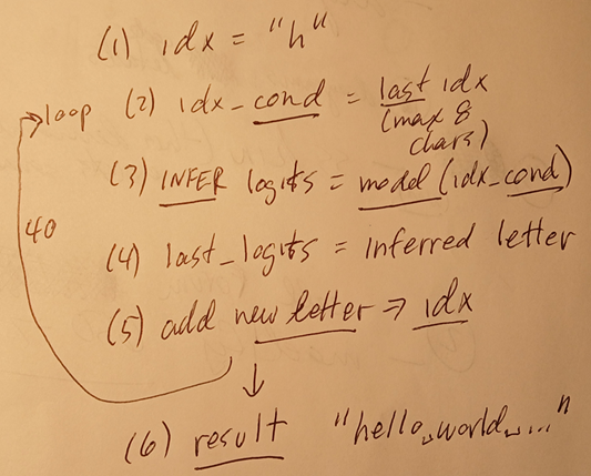
C1 Inference (ch 1)

The diagram below summarizes the inference loop. (my version) this is the inference loop

• (1) idx is the accumulated response in loop z.
• (2) take the last 8 letters of idx as inference input.
• (3) inference of window of idx_cond (1-8 letters). Note: The result is of size idx_cond shifted one letter. forward() is only run for existing letters (which is 1 letter for the first inference; 8 max).
• (4) select last token from the embeddings.
• (5) add the last token of result (new token) to idx.
• (6) after 40 tokens added: join to final result.

GPT feedback

Key idea:
- forward() does not create a longer sequence.
- forward() only computes predictions for the existing input positions.

Example first loop:

idx_cond = [h]
logits shape = [1,1,vocab_size]
last_logits = prediction after h
next_id = e
idx becomes [h,e]

Second loop:

idx_cond = [h,e]
logits shape = [1,2,vocab_size]
last_logits = prediction after e
next_id = l
idx becomes [h,e,l]

C2 Training (ch 2)

This is my simplified, common sense (no jargon) summary of training (it took me a while to get GPT to agree with me):
1. The model (transformer0 makes a prediction.
2. Loss measures how wrong the prediction is.
3. Gradients compute the W/b slopes.
4. The optimizer changes W and b to reduce the loss.
5. Repeat thousands of times.
------------------
I translate AI terminology into engineering terminology:
  gradient      -> W/b slope
  loss          -> prediction error
  parameter     -> W or b
  attention     -> context influence
  logits        -> raw scores

C3 NN init (ch 3)

This part creates (def __init__(self)) the components (matrices) and defines the connections (computations). 
In ch 4 these are used by the forward command (def forward(self,idx)) when running training/inference. 

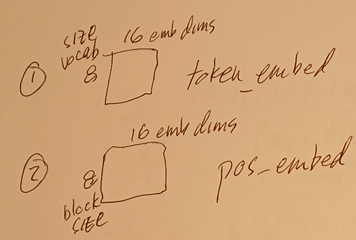
C3.1-2 Matrices for

- token (letter) embedding (16 FP numbers for each letter) (8 letters per batch/sequence)
- position embedding (16 FP numbers for each letter) (8 letters per batch/sequence)

def __init__(self):
    self.token_embed = nn.Embedding(vocab_size, embed_dim)
    self.pos_embed = nn.Embedding(block_size, embed_dim)
def forward(self, idx):
    token_vecs = self.token_embed(idx)
    pos_vecs = self.pos_embed(positions)

C3.3-5 Matrices for

- Weights for QKV (16x16) (used to compute QKV)

def __init__(self):
    self.q = nn.Linear(embed_dim, embed_dim)
    self.k = nn.Linear(embed_dim, embed_dim)
    self.v = nn.Linear(embed_dim, embed_dim)
def forward(self, idx):
    Q = self.q(x)
    K = self.k(x)
    V = self.v(x)

C3.6 FFN NN

- detects complex meaning within the hidden layer 
   (16 FP numbers that were originall the embedding) for a single token (no token mixing).
- much of the structure is hidden behing the libary call 
- token embeddings (16) are input to the h layer "neurons" (64) 
     (h and y are typical naming conventions) 
- h layer outputs are input to the y layer (16) 
- y layer outputs are added to the token hidden layer values (16 FPs) 

def __init__(self):
    self.ffn = nn.Sequential(
        nn.Linear(embed_dim, 64),
        nn.ReLU(),
        nn.Linear(64, embed_dim),         )
def forward(self, idx):
    x = x + self.ffn(x)

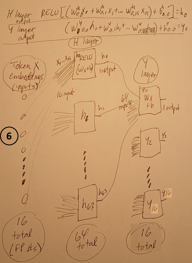
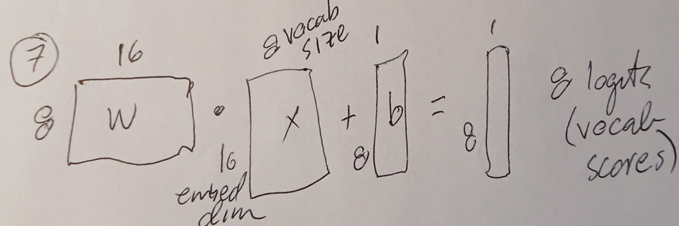
C3.7 Output

- Weights (8x16) dot embed_dims/vocab (16x8) + bias (8x1) = 8 logits 
   (vocab scores for a single token/letter) 

def __init__(self):
    self.out = nn.Linear(embed_dim, vocab_size)
def forward(self, idx):
    logits = self.out(x)

C4 NN forward pass (ch4)

Use components to execute NN algorithms (FOR INFERENCE AND TRAINING).

    def forward(self, idx):

token_vecs, pos_vecs

        B, T = idx.shape
        token_vecs = self.token_embed(idx)
        positions = torch.arange(T, device=device)
        pos_vecs = self.pos_embed(positions)
        x = token_vecs + pos_vecs

context (q,k,v)

        Q = self.q(x)
        K = self.k(x)
        V = self.v(x)
        scores = Q @ K.transpose(-2, -1)
        scores = scores / math.sqrt(embed_dim)
        mask = torch.tril(torch.ones(T, T, device=device))
        scores = scores.masked_fill(mask == 0, float("-inf"))
        weights = F.softmax(scores, dim=-1)
        context = weights @ V
        x = x + context

FFN

        x = x + self.ffn(x)

out

        logits = self.out(x)
        return logits

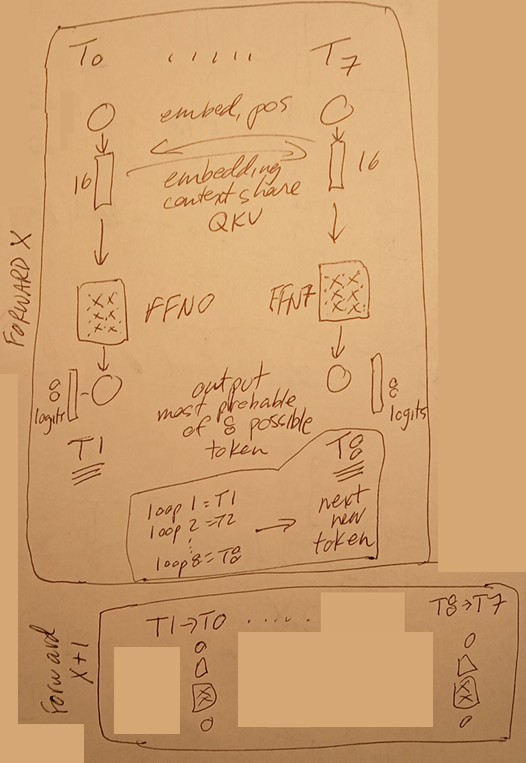
The following diagram shows 
- a forward pass for X with 
  - 8 inputs T0-T7
  - 8 outputs T1-T8 
- T8 is the new token that is added to the running token total
- T1-T8 are the new T0-T7 for the next forward pass X+1  

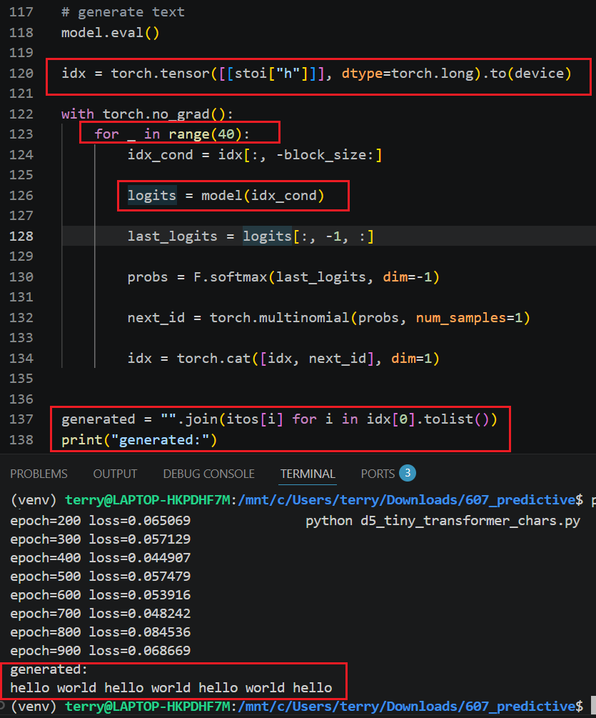
1 Inference

• 1.1 Prompt
• 1.2 Inference loop (40 single letters)
• 1.3 Final response (generated)

Set inference (not training) mode.

model.eval()

1.1 Prompt

use as prompt in loop z+1
Note:  initial prompt is "h"
idx is the accumulated response in loop z

idx = torch.tensor([[stoi["h"]]], dtype=torch.long).to(device)

Suppose: stoi["h"] = 3
Then: idx contains: [[3]], Shape: [B,T] [1,1], Meaning: 1 sequence, 1 token, The prompt is literally: "h".

1.2 Inference loop (40 single letters)

with torch.no_grad():
    for _ in range(40):

no_grad()
generate 40 new tokens One at a time.
Iteration 1: Input: h, Model predicts: e, Append: he
Iteration 2: Input: he, ...

        idx_cond = idx[:, -block_size:]

take the last 8 letters of idx as inference input
= idx[all_rows, last_block_size_columns] [B,T]? (T<=8)
creates the context window.
So if: block_size = 4 then: idx_cond = [[7,8,9,10]]
Example: hello world becomes: lo world for the next prediction.
cond is short for conditioned or conditioning context.
The idea is: idx contains the entire generated sequence so far.
But the model can only look at the last block_size tokens:

1.2.1 forward pass (inference of single letter)

Note: The result is of size idx_cond shifted one letter.
THE KEY POINT I WAS MISSING: 
forward() has the idx_cond as parameter which has 1-8 letters.
so forward() is only run for existing letters 
(which is 1 letter for the first inference; 8 max)

        logits = model(idx_cond)

Suppose:
idx_cond = [[5, 2, 7, 1]]
Then: logits = model(idx_cond) might return:
logits.shape = [1, 4, 8]
meaning:
•	1 sequence
4 token positions
8 vocabulary entries
The model has produced predictions for every position:
•	position 0 predicts token 1
position 1 predicts token 2
position 2 predicts token 3
position 3 predicts token 4

        last_logits = logits[:, -1, :]

= 2 dimensions, not 3.  [B, T, C] -> [B, C]
for generation we only care about the newest position:
Give me the prediction for the last token position.

        probs = F.softmax(last_logits, dim=-1)

dim=-1 means last dimension
apply softmax across the vocabulary dimension (C?)

        next_id = torch.multinomial(probs, num_samples=1)

chooses the next token.
Let's assume: probs = [[0.10, 0.05, 0.70, 0.15]]
Meaning: token 0 : 10% ....
Randomly pick according to the probabilities.
might return: [[2]] most of the time because token 2 has probability 0.70.
Occasionally: [[0]] or [[3]]
num_samples=1 Means: Pick one token.
Result shape: next_id.shape = [1, 1]
Example: next_id = [[2]]
Why not just take the biggest?
You could do: next_id = torch.argmax(probs, dim=-1, keepdim=True)
which would always pick: the highest probability token
But then generation becomes very deterministic.
Shape walkthrough
Before: probs.shape = [1, 8]
(one batch, 8 vocabulary probabilities)
After: next_id = torch.multinomial(probs, 1)
you get: next_id.shape = [1, 1]
because you've chosen: 1 token for 1 batch
Example: next_id = [[5]] meaning: Token #5 was selected.
ME: but the result has always been "hello world hel..."
Yes — that is normal for a tiny demo.
So probs may look like: token "e" = 0.98, all others = tiny
Then multinomial is “random,” but it almost always chooses "e".

        idx = torch.cat([idx, next_id], dim=1)

This line appends the newly generated token to the sequence.
Suppose before generation step: idx = [[1, 2, 3, 4]] Shape: [1, 4]
And suppose: next_id = [[5]] Shape: [1, 1]
torch.cat([tensor1, tensor2], dim=1)
means: Join tensor1 and tensor2 along dimension 1
idx shape = [B, T] B = batch T = token positions

1.3 Final response (generated)

after 40 tokens added: join to final result

generated = "".join(itos[i] for i in idx[0].tolist())
print("generated:")
print(generated)

It converts: token IDs  > characters > string
Suppose after generation: idx = [[3, 2, 5, 5, 7]]  Shape: [1, 5]
idx[0] means: Take batch 0 Result: tensor([3, 2, 5, 5, 7]) Shape: [5]
idx[0].tolist() converts the tensor into a normal Python list: [3, 2, 5, 5, 7]
itos means: integer to string (the reverse of stoi, string to integer)
itos[i] for i in idx[0].tolist() loops through: [3, 2, 5, 5, 7] and produces 'h' 'e' ...
"".join(...) means: Join all strings together with nothing between them
For your tiny transformer: idx = [[3,2,4,4,5,0,7,5,6,4,1]] > ['h','e','l','l','o',' ','w','o','r','l','d']

2 Training

• 2.1 model, loss_fn, optimizer  
• 2.2 prepare training data 
• 2.3 training loop (1000 epochs)

2.1 Model, loss_fn, optimizer

model = TinyTransformer().to(device)

Move all weights to CPU or GPU.
creates an instance of the class: class TinyTransformer(nn.Module):
model = variable that points to the transformer object.

loss_fn = nn.CrossEntropyLoss()	

(ME: specify the nn loss function).
Measure prediction error.
Low probability assigned to correct token → high loss
High probability assigned to correct token → low loss
actual next character = "o"
model predicts:  space=0.01,  d=0.02,  e=0.05  ...  o=0.90  → low loss

optimizer = torch.optim.Adam(model.parameters(), lr=0.01)

(ME: specify the) Training algorithm.
Uses gradients from backprop to adjust all trainable weights:
embeddings, position embeddings, Q/K/V weights, FFN weights, output layer weights
(see section 3 "NN algorithm" for details). 

 

2.2 Prepare training data

text = "hello world hello world hello world "

This is the training data (all of it).

chars = sorted(list(set(text)))

build the vocabulary.
set(text)
Suppose: text = "hello world"
Then: set(text) extracts unique characters: {'h','e','l','o',' ','w','r','d'}
Duplicates removed.
list(set(text)) converts set to list: ['h','e','l','o',' ','w','r','d']
Order is arbitrary.
chars = sorted(list(set(text)))
sorts characters: [' ', 'd', 'e', 'h', 'l', 'o', 'r', 'w']
Now vocabulary ordering is deterministic.

vocab_size = len(chars)

Counts unique characters: 8 for this example.

stoi = {ch: i for i, ch in enumerate(chars)}

This is the simplest possible tokenizer.
means: string to integer lookup table
text = "hello world"
Unique characters: chars = sorted(list(set(text)))
might become: [' ', 'd', 'e', 'h', 'l', 'o', 'r', 'w']
Result: { ' ': 0,  'd': 1,  'e': 2,  'h': 3,  'l': 4,  'o': 5,  'r': 6,  'w': 7}
So: stoi['h'] returns: 3

itos = {i: ch for ch, i in stoi.items()}

creates the reverse mapping: integer to string
Result: { 0: ' ', 1: 'd', 2: 'e', 3: 'h', 4: 'l', 5: 'o', 6: 'r', 7: 'w'}
So: itos[3] returns: 'h'

data = torch.tensor([stoi[ch] for ch in text], dtype=torch.long).to(device)

This converts the training text into token IDs.
Suppose: text = "hello"
and: stoi = { 'e':0, 'h':1, 'l':2, 'o':3 }
[stoi[ch] for ch in text] and produces: [1, 0, 2, 2, 3]
Then: torch.tensor(...) converts that Python list into a tensor: tensor([1,0,2,2,3])
Then: dtype=torch.long means: 64-bit integer tensor (PyTorch embeddings require integer token IDs).
Then: .to(device) moves tensor to: GPU (cuda) or CPU depending on: device
This tensor is the transformer's equivalent of the MNIST image tensor from D4.

block_size = 8

X.shape becomes: [batch_size, 8]
For your demo: [16, 8]
meaning: 16 training sequences, 8 tokens per sequence
Conceptually: block_size is the transformer's: memory window / context length
The model can attend only to: the previous 8 tokens
Real models: D5 demo: block_size = 8, GPT-2: 1024, Llama: 4096+

embed_dim = 16

Each character has a learned embedding:
h → [0.2, -1.1, ..., 0.7], e → [1.3,  0.4, ..., -0.2] ....
Each vector contains: 16 numbers

2.3 training loop (1000 epochs)

SUBSECTIONS
- 2.3.0 Get batch of input/output block pairs 
- 2.3.1 Run input block X through the model (model(X))
- 2.3.2 Compute prediction error (loss_fn())
- 2.3.3 Compute W/b (param) slopes (loss.backward())
- 2.3.4 Update W/b params (optimizer.step())

num_epochs = 1000
for epoch in range(num_epochs):

(loop 1000 times)

2.3.0 Get batch of input/output block pairs

Get a batch (16) of input/output letter block pairs X/Y (size=8) with random start positions

    X, Y = get_batch()

(def get_batch())

    ix = torch.randint(0, len(data) - block_size - 1, (16,), device=device)

picks random training positions from the text.
for "hello world hello world hello world"
Suppose: len(data) = 36 block_size = 8
Then: torch.randint(    0,    27,    (16,))
means: generate 16 random integers between 0 and 26
Example: [5, 12, 3, 20, 1, 17, 9, ...]
Why?Because later:
X = data[i:i+block_size] needs room for: 8 input tokens + 1 target token
So if: i = 26 then: 26 ... 34 still fits inside the text.
The result: ix.shape is: [16] meaning: 16 random starting positions for the training batch.

    X = torch.stack([data[i:i + block_size] for i in ix])
    Y = torch.stack([data[i + 1:i + block_size + 1] for i in ix])
    return X, Y

Suppose text is: hello world
and token IDs are: 
h e l l o _ w o r l d
1 2 3 3 4 0 5 4 6 3 7
Suppose:block_size = 4
and one random position is: i = 0
X
data[i:i+block_size]
becomes: data[0:4] which is: h e l l
So: X contains: h e l l
Y
data[i+1:i+block_size+1]
becomes: data[1:5] which is: e l l o
So: Y contains: e l l o
Therefore the training pair is: X: h e l l , Y: e l l o
Meaning:given h predict e , .... , given l predict o
After stacking 16 random examples:
X.shape becomes: [16,8]
and: Y.shape becomes: [16,8]
Meaning: 16 training sequences, 8 tokens each
This is the transformer's equivalent of D4's: 64 images + 64 labels
except now it is: 16 sequences + 16 shifted target sequences

(continue epochs loop)

2.3.1 Run input block X through the model (model(X))

Make a "forward pass".
X = input.
Y = target.

    logits = model(X)

for: model(X) PyTorch automatically calls: model.forward(X) behind the scenes.
So yes, both references (model = Tiny....) are pointing to the same transformer instance.
The first line creates it. The second line uses it.

    B, T, C = logits.shape

shape is: [16,8,8] 16 sequences, 8 token positions, 8 vocabulary outputs
B = Batch size, T = Token positions, C = Classes (vocabulary size)
Visualize one sequence:
Position 0: [8 logits]
Position 1: [8 logits]
...

2.3.2 Compute prediction error (loss_fn())

Compare model output to block Y. 
loss = prediction error

loss = loss_fn( 
   logits.reshape(B * T, C), 
   Y.reshape(B * T), )

Compute CrossEntropy loss for the 128 next-token predictions.
loss_fn = nn.CrossEntopyLoss()
nn.CrossEntropyLoss() expects:
- predictions: [number_of_examples, number_of_classes]
- targets: [number_of_examples]
So we flatten: logits.reshape(B*T, C)
which becomes: [128,8] because: 16 × 8 = 128
Interpretation: 128 next-character predictions, 8 possible output characters
Similarly: Y.reshape(B*T) becomes: [128]
Example: [2,4,4,5,0,7,5,6, ...] where each number is: the correct next token ID
So CrossEntropyLoss sees:
Prediction #1: 8 logits Target = 2
Prediction #2: 8 logits Target = 4 ...
Prediction #128: 8 logits Target = 6

2.3.3 Compute W/b (param) slopes (loss.backward())

Make a "backward pass" that computes ∂loss/∂parameter (gradients).

optimizer.zero_grad()

after optimizer.step() updates the weights: the gradients are still there!
PyTorch does not automatically clear them.
Why is that a problem? Suppose next batch:
loss.backward() produces: new gradient = 0.30
PyTorch accumulates: W.grad = 0.15 + 0.30 instead of: W.grad = 0.30
So gradients would keep growing every iteration.

loss.backward()

This is the line that starts backpropagation.
Compute gradients for every trainable parameter.
Example: loss = 0.058
After: loss.backward()
PyTorch walks backwards through the entire computation graph and computes:
∂loss/∂parameter for every trainable parameter.
Examples: ∂loss/∂token_embedding, /∂position_embedding, /∂Wq, /∂bq, /∂Wk, /∂Wv, /∂FFN weights, /∂output weights
Conceptually: If I increase this weight slightly, does the loss go up or down? The answer is stored as the gradient.
Nothing is changed yet. It only computes gradients. so Adam can later update them.
"determine blame" description is actually a pretty good mental model.
The transformer has millions (or in D5, thousands) of parameters.

2.3.4 Update W/b params (optimizer.step())

optimizer.step()

Updates the trainable parameters.
  W = W - lr * W.grad
  b = b - lr * b.grad
Example:
  W = 2.0
  grad = 0.15
  lr = 0.1
new W = 2.0 - 0.1*0.15 = 1.985
The real Adam algorithm is more sophisticated, but this is the basic idea.

3 NN initialization (__init__) (create components / define matrices)

• 3.1 token and position embeddings
• 3.2 QKV content influence
• 3.3 FFN
• 3.4 output logits

creates the trainable components
"What is the network made of?"
= define matrices
exactly how PyTorch models are structured.

class TinyTransformer(nn.Module):
    def __init__(self):
        super().__init__()

3.1 token and position embeddings

        self.token_embed = nn.Embedding(vocab_size, embed_dim)  ##8,16

initialize with random values.

        self.pos_embed = nn.Embedding(block_size, embed_dim)  ##8,16

creates the embedding table and initializes it with random values.
ME: so just coincidence that blocksize and vocab size both = 8
Yes. Pure coincidence.

3.2 QKV content influence

so the following code sets up or defines (somehow) the QKV mechanism.

        self.q = nn.Linear(embed_dim, embed_dim)
        self.k = nn.Linear(embed_dim, embed_dim)
        self.v = nn.Linear(embed_dim, embed_dim)

For a single attention head with:
embed_dim = 16
you have: Wq : 16x16, Wk : 16x16, Wv : 16x16
          bq : 16x1, bk : 16x1, bv : 16x1
3 matrices 16x16, 3 bias vectors 16x1
same Wq, Wk, Wv are used for every token.
no biases in the equations because most transformer explanations omit them:
biases usually not important for QKV, so authors often leave them out to simplify.
for nn.Linear, the bias is there unless: nn.Linear(embed_dim, embed_dim, bias=False)

3.3 FFN

        self.ffn = nn.Sequential(
            nn.Linear(embed_dim, 64),
            nn.ReLU(),
            nn.Linear(64, embed_dim),
        )

ME: 
h1 (hidden layer) has 64 neurons.
 16 inputs to each neuron.
 RELU(Wx+b) for each output.  bias is a single scalar.
h2 (hidden layer) has 16 neurons.
 64 inputs to each neuron.
 (Wx+b) for each output.  bias is a single scalar.

embed_dim = 16
Layer h1 nn.Linear(16, 64)
64 neurons, 16 inputs per neuron
Each neuron computes: Wx + b , W = 1x16, x = 16x1, b = scalar
Then: ReLU(Wx+b) produces one output. So h1 has:64 outputs
Layer h2 nn.Linear(64, 16)
16 neurons, 64 inputs per neuron
Each neuron computes: Wx + b
where: W = 1x64, x = 64x1, b = scalar
No ReLU after this layer.
So h2 produces: 16 outputs
total of: 80 bias values

3.4 output logits

     self.out = nn.Linear(embed_dim, vocab_size)

with: embed_dim = 16 vocab_size = 8
PyTorch creates:
Wout : 8x16, bout : 8x1
Given: x = h2 output = 16x1
the outputs are: y0 = W0·x + b0, y1 = W1·x + b1, y2 = W2·x + b2 ... y7 = W7·x + b7
Each yi is a scalar.
Collect them together: [y0 y1 y2 y3 y4 y5 y6 y7]ᵀ
and you get: 8x1 which is the logits vector.
So your interpretation is exactly right:
16 hidden values > 8 output neurons > 8 logits > one logit per vocabulary token
This is the "unembedding" layer that converts the final hidden state into scores for the 8 possible next characters.

4 NN forward pass (forward(self, idx)) (use components to execute algorithms)

• 4.1 token/pos embed
• 4.2 QKV context sharing (“attention heads”)
• 4.3 FFN
• 4.4 Out logits

uses the trainable components
"What calculations does the network perform?"
execute algorithm
exactly how PyTorch models are structured.

    def forward(self, idx):

defines: how data flows through the network. exactly like D4.
D4: image  → conv       → relu      → pool → fc
D5: tokens → embeddings → attention → FFN  → logits

B = 16  batches
T = 8   token positions
C = 16  embedding dimensions
Everything in forward() is operating on the entire batch at once.

4.1 token/pos embed

        B, T = idx.shape

[16, 8] meaning:
16 sequences , 8 tokens per sequence
In transformer terminology:
B = batch size
T = sequence length (tokens)
C = channels/features/embedding dimension
Later you'll see tensors like: [B,T,C] [16,8,16]

4.1.0 Initial token representations (4 lines)

These four lines are the transformer's equivalent of: loading the image into the CNN.
They create the initial token representations.

4.1.1 Step 1 token_vecs

        token_vecs = self.token_embed(idx)   # 16,8,16

Suppose: idx shape: [16,8]
Example row: [3,2,4,4,5,0,7,5]
which means: h e l l o _ w o
Each token ID is looked up in the embedding table.
Since: embed_dim = 16 each token becomes: 16 numbers
Result: token_vecs shape: [16,8,16]
Meaning: 16 sequences, 8 tokens, 16-dimensional vector per token

4.1.2 Step 2 positions

        positions = torch.arange(T, device=device)

Since: T = 8 this creates: [0,1,2,3,4,5,6,7]
These are: token positions

4.1.3 Step 3 pos_vecs

        pos_vecs = self.pos_embed(positions)

does not create new random values. It performs a lookup.
NOTE: pos vector initial random, then trained
Each position gets its own learned vector.
Example: 
position 0 → [0.1, -0.3, ...]
position 1 → [1.2, 0.5, ...]
position 2 → [-0.7, 0.8, ...]
Shape: [8,16]

4.1.4 Step 4 x

        x = token_vecs + pos_vecs

This is one of the most important lines in a transformer.
NOTE: pytorch broadcast used for changing pos_vecs to [16,8,16] (copies across all batches)
Suppose: token embedding for "h": [2,5,1,...]
and: position 0 embedding: [10,20,30,...]
Then: x = [12,25,31,...] Simple vector addition.
Why? Without positions:
h e l l o
o l l e h
would look like the same bag of tokens. Attention itself does not know order. 
Position embeddings provide: where each token is located
Final shape:
x shape: [16,8,16]
Meaning: B = 16, T = 8, C = 16
This tensor x is now the transformer's equivalent of the CNN feature maps.
It is the representation that gets fed into:
Q = self.q(x), K = self.k(x), V = self.v(x)
which is where the attention mechanism begins.

4.2 QKV context sharing (“attention heads”)

for chats, in docx #607 search for "QKV@1", "QKV@2" (@2 is final discussion).

4.2.1 SImplified explanation of algorithm execution

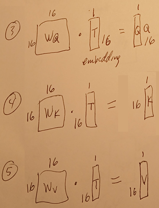
4.2.1.1 Step 1

Compute Q0...Q7 and K0...K7.
Q0 = Wq · emb0 (embedding for letter 0), K1 = Wk · emb0, etc
1x16 dot 16x1 = scalar (plain number).
This basically determines the Q and K for each letter based on the embedding values (16) of that letter.

4.2.1.2 Step 2

Compute all combinations of Q0...Q7 · K0...K7. 
For example, compare Token (letter) 0 against all (8) tokens (including itself):
Q0K0 = Q0ᵀ · K0, Q0K1 = Q0ᵀ · K1, Q0K2 = Q0ᵀ · K2 ...
Example values: Q0K0 = 2.1, Q0K1 = 4.5, Q0K2 = 1.2.
NOTE: Q0K1 = the level that token token1 will influencce the context (16 embeddings) of token0. Token 0 is the target.

4.2.1.3 Step 3

Determine which token(s) influence each token the most.
We want to "exaggerate" the 1-2 highest scores and minimize all others.
For that we use Softmax.
A00 = softmax(Q0K0), A01 = softmax(Q0K1), A02 = softmax(Q0K2)
Example: A00 = 0.08, A01 = 0.80, A02 = 0.12
These are the attention weights for token 0.

4.2.1.4 Step 4

Now compute the context values for all tokens.
V0 = Wv · emb0, V1 = Wv · emb1, V2 = Wv · emb2
Each is: 16x16 dot 16x1 = 16x1.

4.2.1.5 Step 5

Compute context for token 0:
context0 = A00·V0 + A01·V1 + A02·V2...
This is the key result.
If: A01 = 0.80 then token 1 contributes heavily to: context0.

4.2.2 Matrix multiplication descriptions

This does the everything described in 4.2.1 and more, but describes in matrix format.

        Q = self.q(x)
        K = self.k(x)
        V = self.v(x)

1) compute 8 sets of q,k,v .. all use the same method
(16x16 W matrix) dot (16x1 token) + bias (16x1) = q, k, v (16x1) for all 8 tokens
Q.shape = [16,8,16], K.shape = [16,8,16], V.shape = [16,8,16]
[sequence, tokens, Q/K/V values]

        scores = Q @ K.transpose(-2, -1)
        scores = scores / math.sqrt(embed_dim)

2) Compute [ K(transpose) dot Q ] for all token-token pairs (including "self pairing").
Result: for each pair one scalar (just call these QK values).
value belong to the Q token (letter).
More details:
code wants all 64 scores at once:
Q0K0 Q0K1 ... Q0K7
Q1K0 Q1K1 ... Q1K7
...
Q7K0 Q7K1 ... Q7K7
So we arrange the matrices:
Q = [8,16] , K = [8,16]
and compute:
scores = Q @ K.T
Now:
Q     = [8,16]
K.T   = [16,8]
Therefore:
[8,16] @ [16,8]
          ↓
       [8,8]

3) compute softmax(KQ)s (call these results KQm , m = softMax) 
to determine (context) info sharing between each token pair (including self pairs). 
do not share between future tokens (letters).
T = # of tokens.

        mask = torch.tril(torch.ones(T, T, device=device))
        scores = scores.masked_fill(mask == 0, float("-inf"))

Wherever mask==0, replace score with -∞.
3  -∞  -∞  -∞
1   7  -∞  -∞
2   6   3  -∞
8   1   2   4

        weights = F.softmax(scores, dim=-1)

Example: row 2 [2, 6, 3, -∞]
Softmax produces: [0.017, 0.936, 0.047, 0.0]

        context = weights @ V

4) add weight * V (16x1) for all 16 context contributions to a token. 
repeat for all token pairs.
(weight = KQm (scalar) (m=softmax))
tiny example.
Suppose: weights [0.1, 0.2, 0.7]
Meaning: 10% attention to token0, 20% attention to token1, 70% attention to token2
Suppose: V0 = [1,2], V1 = [5,6], V2 = [10,20]
Then: context = 0.1*V0 + 0.2*V1 + 0.7*V2
Compute:
0.1*[1,2]   = [0.1,0.2]
0.2*[5,6]   = [1.0,1.2]
0.7*[10,20] = [7.0,14.0]
Add: context = [8.1,15.4]
This is a new vector. Created by combining information from multiple tokens.

        x = x + context

add the contributions
performed for the entire batch:
batch 0:     x0 = x0 + context0
batch 1:     x1 = x1 + context1
...
batch 15:     x15 = x15 + context15

4.3 FFN

        x = x + self.ffn(x)

The FFN is just applying the same learned detector network to every token in parallel. 
128 independent FFN evaluations / simultaneously on the GPU.
for all 128 tokens. performs large matrix operations on the entire tensor:
[16,8,16]
    ↓ Linear(16,64)
[16,8,64]
    ↓ ReLU
[16,8,64]
    ↓ Linear(64,16)
[16,8,16]

4.4 Out logits

        logits = self.out(x)
        return logits 

This is the final prediction layer.
x.shape = [16, 8, 16] 16 batches, 8 token positions, 16 hidden dimensions
self.out = nn.Linear(16, 8) (embed_dim, vocab_size) applied to every token.
So: [16, 8, 16] -> Linear(16,8) -> [16, 8, 8]
logits.shape = [16, 8, 8] 16 sequences, 8 token positions, 8 vocabulary scores
[2.1, 0.3, 4.5, 1.2, -0.7, 3.0, 0.1, 1.8]
Those are the scores for the 8 possible next characters.

26.0603 (v1 26.0601)