2.2.1 D4 CNN image classifier
WIP. Runs locally and on Render (CPU mode). Input from MNist.
See also
TOC
- 1 Output
- 2 PY scripts
- 3 Render deploy
- 4 Code with detailed comments. Great commentary for each line of the code (from GPT). Study this closely to understand the gist.
1 Output
python d4_tiny_cnn_mnist.py
device: cuda
epoch=0 loss=353.2148 accuracy=0.8866
epoch=1 loss=94.7172 accuracy=0.9690
test accuracy=0.9786
2 PY scripts
- d4_tiny_cnn_mnist.py
- d4_api_mnist.py (for Render)
- d4_test_api.py (for Render)
3 Render deploy
Add deploy details.
4 Code with detailed comments
TOC
- 4.1 d4_tiny_cnn_mnist.py
- 4.2 d4_api_mnist.py
- 4.3 d4_test_api.py
4.1 d4_tiny_cnn_mnist.py
# -----------------------------
# D4 Tiny CNN Image Classifier
# -----------------------------
transform = transforms.ToTensor()
This converts MNIST images into PyTorch tensors.
MNIST images originally come as:
PIL images
basically standard image objects.
But the CNN expects:
torch tensors
So:
transform = transforms.ToTensor()
means:
before giving image to NN:
convert image → tensor
________________________________________
Important conversion
MNIST grayscale images are:
28 × 28 pixels
ToTensor() converts them into:
[1,28,28]
tensor shape.
Meaning:
[channel,height,width]
where:
1 = grayscale channel
________________________________________
Also rescales pixel values
Original image pixels:
0 → 255
ToTensor() converts to:
0.0 → 1.0
floating-point values.
Very important for NN training stability.
________________________________________
So mechanically
image file
↓
ToTensor()
↓
normalized tensor
↓
CNN input
rain_data = datasets.MNIST(
    root="data",
    train=True,
    download=True,
    transform=transform,
)
This loads the MNIST training dataset.
train_data = datasets.MNIST(...)
creates an object representing:
60,000 handwritten digit images
________________________________________
root="data"
root="data"
means:
store dataset files
inside ./data directory
________________________________________
train=True
train=True
means:
load TRAINING split
MNIST has:
60k training images
10k test images
________________________________________
download=True
download=True
means:
automatically download dataset
if not already present
________________________________________
transform=transform
transform=transform
means:
before returning image:
apply ToTensor()
So each image becomes:
tensor shape:
[1,28,28]
instead of raw PIL image.
________________________________________
Important conceptual point
train_data is NOT yet:
a tensor batch
It is more like:
dataset object
that can provide samples.
Example:
X, Y = train_data[0]
returns:
X = image tensor
Y = digit label
Example label:
7
test_data = datasets.MNIST(
    root="data",
    train=False,
    download=True,
    transform=transform,
)
Same idea — but this loads the TEST dataset instead of training dataset.
train=False
means:
load MNIST test split
which contains:
10,000 unseen images
These images are NOT used during training.
Very important concept:
training data
=
learn weights
test data
=
evaluate generalization
So later:
for X, Y in test_loader:
checks:
can the CNN classify
new unseen digits?
That is why:
test accuracy
is meaningful.
train_loader = DataLoader(train_data, batch_size=64, shuffle=True)
test_loader = DataLoader(test_data, batch_size=64, shuffle=False)
DataLoader creates an iterator that feeds batches to the CNN during training/testing.
Without DataLoader:
you would manually extract samples
With DataLoader:
PyTorch automatically provides batches
________________________________________
train_loader
train_loader = DataLoader(
    train_data,
    batch_size=64,
    shuffle=True
)
means:
during training:
- take 64 images at a time
- randomize order each epoch
________________________________________
batch_size=64
Each training step receives:
64 images
64 labels
Tensor shapes become:
X:
[64,1,28,28]

Y:
[64]
Meaning:
[batch,channel,height,width]
________________________________________
shuffle=True
Important for training.
randomize sample order each epoch
This helps:
better generalization
less training bias
________________________________________
test_loader
shuffle=False
because testing does NOT require randomization.
You only want:
stable evaluation
________________________________________
Conceptually
DataLoader does:
dataset
↓
mini-batches
↓
training loop
Very central PyTorch abstraction.
class TinyCNN(nn.Module):
    def __init__(self):
        super().__init__()
        self.conv1 = nn.Conv2d(1, 8, kernel_size=3, padding=1)
        self.conv2 = nn.Conv2d(8, 16, kernel_size=3, padding=1)
        self.pool = nn.MaxPool2d(2, 2)
        self.fc1 = nn.Linear(16 * 7 * 7, 64)
        self.fc2 = nn.Linear(64, 10)
This defines the CNN architecture.
Mechanistically:
image
↓
conv layer
↓
conv layer
↓
flatten
↓
fully connected layers
↓
10 digit outputs
________________________________________
class TinyCNN(nn.Module)
class TinyCNN(nn.Module):
defines a custom neural network.
nn.Module is PyTorch base class for all NNs.
________________________________________
super().init()
Initializes internal PyTorch NN machinery.
Standard boilerplate.
________________________________________
conv1
self.conv1 = nn.Conv2d(
    1,
    8,
    kernel_size=3,
    padding=1
)
means:
1 input channel
↓
8 learned filters
↓
3x3 kernels
Input image:
[1,28,28]
Output becomes:
[8,28,28]
Meaning:
8 feature maps
________________________________________
conv2
self.conv2 = nn.Conv2d(
    8,
    16,
    kernel_size=3,
    padding=1
)
means:
8 input feature maps
↓
16 new filters
↓
16 output feature maps
Output:
[16,14,14]
(after pooling later)
________________________________________
pool
self.pool = nn.MaxPool2d(2,2)
means:
reduce spatial resolution by 2
Example:
28x28 → 14x14
14x14 → 7x7
Pooling keeps strongest activations.
________________________________________
fc1
self.fc1 = nn.Linear(
    16*7*7,
    64
)
FC = FULLY CONNECTED (SEE BELOW)
After conv/pooling:
16 feature maps
each 7x7
Flattened into:
16×7×7 = 784 values
Then fully connected layer:
784 → 64
________________________________________
fc2
self.fc2 = nn.Linear(64,10)
Final classifier:
64 hidden features
↓
10 digit logits
representing:
0 1 2 3 4 5 6 7 8 9

ME: what does fc mean?
fc means:
fully connected
Same thing as:
dense layer
linear layer
So:
self.fc1
self.fc2
are standard feedforward NN layers like your earlier D1/D2 demos.
________________________________________
Why “fully connected”?
Because:
every output neuron
connects to every input value
Example:
784 inputs
→
64 outputs
means:
784 × 64 weights
Very different from convolution layers, where connections are local:
3x3 neighborhood only
instead of:
all-to-all connections
    def forward(self, x):
        x = self.pool(F.relu(self.conv1(x)))  # [batch, 8, 14, 14]
        x = self.pool(F.relu(self.conv2(x)))  # [batch, 16, 7, 7]
        x = x.reshape(x.size(0), -1)          # [batch, 784]
        x = F.relu(self.fc1(x))               # [batch, 64]
        x = self.fc2(x)                       # [batch, 10]
        return x
This is the actual CNN execution pipeline.
Input:
x shape:
[batch,1,28,28]
Meaning:
[batch,channel,height,width]
________________________________________
conv1 → relu → pool
x = self.pool(
        F.relu(
            self.conv1(x)
        )
    )
Step-by-step:
________________________________________
conv1
[batch,1,28,28]
↓
[batch,8,28,28]
8 learned filters produce:
8 feature maps
________________________________________
relu
Negative values become zero.
________________________________________
pool
28x28
↓
14x14
So final shape:
[batch,8,14,14]
________________________________________
conv2 → relu → pool
x = self.pool(
        F.relu(
            self.conv2(x)
        )
    )
Now:
[batch,8,14,14]
↓
[batch,16,14,14]
↓
[batch,16,7,7]
Meaning:
16 learned feature maps
________________________________________
flatten
x = x.reshape(x.size(0), -1)
This converts:
[batch,16,7,7]
into:
[batch,784]
because:
16×7×7=784
CNN spatial structure is flattened into vector.
________________________________________
fc1
x = F.relu(self.fc1(x))
Standard feedforward layer:
784 → 64
________________________________________
fc2
x = self.fc2(x)
Final classifier:
64 → 10
Output shape:
[batch,10]
representing logits for digits:
0 1 2 3 4 5 6 7 8 9
________________________________________
return x
Returns final logits.
Softmax NOT yet applied.
CrossEntropyLoss handles that internally.
model = TinyCNN().to(device)
loss_fn = nn.CrossEntropyLoss()
optimizer = torch.optim.Adam(model.parameters(), lr=0.001)
These are the three core training objects:
model
loss function
optimizer
________________________________________
model
model = TinyCNN().to(device)
creates the CNN instance and moves it to:
GPU or CPU
depending on:
device
________________________________________
loss function
loss_fn = nn.CrossEntropyLoss()
defines:
how wrong predictions are measured
For MNIST:
10 competing digit classes
So CrossEntropy is appropriate.
________________________________________
optimizer
optimizer = torch.optim.Adam(
    model.parameters(),
    lr=0.001
)
defines:
how weights get updated
during training.
________________________________________
Big picture
Training loop becomes:
images
↓
CNN forward pass
↓
logits
↓
CrossEntropy loss
↓
backprop gradients
↓
Adam updates weights
# Train
num_epochs = 2
for epoch in range(num_epochs):
    model.train()
puts the CNN into:
training mode
Important because some layers behave differently during:
training
vs
inference
Especially:
Dropout
BatchNorm
Your current CNN does NOT use those layers,
so here:
model.train()
does not visibly change much.
But it is standard/important practice.
________________________________________
Similarly later:
model.eval()
puts model into:
inference/evaluation mode
Very important in larger CNNs and transformers.
    total_loss = 0
    correct = 0
    total = 0
    for X, Y in train_loader:
        X = X.to(device)
        Y = Y.to(device)
        logits = model(X)
        loss = loss_fn(logits, Y)
        optimizer.zero_grad()
        loss.backward()
        optimizer.step()
        total_loss += loss.item()

```output
train_loader = DataLoader(train_data, batch_size=64, shuffle=True)
loss is a PyTorch tensor.
Example:
tensor(0.8421, device='cuda:0')
But:
loss.item()
extracts the plain Python number:
0.8421
________________________________________
So:
total_loss += loss.item()
means:
accumulate scalar losses
across batches
during the epoch.
________________________________________
Important:
loss
is a tensor participating in autograd.
loss.item()
is just a plain numeric value for logging/statistics.
        pred = logits.argmax(dim=1)
        correct += (pred == Y).sum().item()
        total += Y.size(0)

```output
This computes training accuracy.
________________________________________
predicted classes
pred = logits.argmax(dim=1)
logits shape:
[batch,10]
Example row:
[ -2.1, 5.3, 0.7, ... ]
argmax(dim=1) selects:
index of largest logit
Example:
5.3 largest
→ predicted digit = 1
So:
pred
contains predicted digits for whole batch.
Shape:
[batch]
________________________________________
compare predictions vs truth
(pred == Y)
Example:
pred:
[1,7,2,9]

Y:
[1,3,2,8]
Result:
[True, False, True, False]
________________________________________
count correct
.sum()
becomes:
2
Then:
.item()
converts tensor → Python number.
So:
correct += ...
accumulates:
total correct predictions
across batches.
________________________________________
total samples
total += Y.size(0)
Y.size(0) means:
batch size
Usually:
64
So:
total
tracks:
total images processed
________________________________________
    accuracy = correct / total
    print(f"epoch={epoch} loss={total_loss:.4f} accuracy={accuracy:.4f}")
final accuracy
Later:
accuracy = correct / total
Example:
9822 / 10000
=
0.9822
# Test
model.eval()
correct = 0
total = 0
with torch.no_grad():
    for X, Y in test_loader:
        X = X.to(device)
        Y = Y.to(device)
        logits = model(X)
        pred = logits.argmax(dim=1)
        correct += (pred == Y).sum().item()
        total += Y.size(0)
print(f"test accuracy={correct / total:.4f}")

# Show one prediction
X_sample, Y_sample = test_data[0]
with torch.no_grad():
    logits = model(X_sample.unsqueeze(0).to(device))
    pred = logits.argmax(dim=1).item()
This runs inference on ONE test image.
________________________________________
get one MNIST sample
X_sample, Y_sample = test_data[0]
returns:
X_sample:
image tensor

Y_sample:
correct digit label


Shapes:
X_sample:
[1,28,28]

Y_sample:
scalar integer
Example:
Y_sample = 7
________________________________________
no_grad
with torch.no_grad():
means:
inference only
no backprop
________________________________________
unsqueeze(0)
X_sample.unsqueeze(0)
adds batch dimension.
Before:
[1,28,28]
After:
[1,1,28,28]
Meaning:
[batch,channel,height,width]
CNN expects batch dimension even for one image.
________________________________________
model inference
logits = model(...)
Output shape:
[1,10]
Meaning:
1 image
10 digit logits
Example:
[
 [-4.1, -2.7, ..., 8.9, ...]
]
________________________________________
argmax
pred = logits.argmax(dim=1).item()
selects:
largest logit index
Example:
largest value at index 7
So:
pred = 7
Final predicted digit.
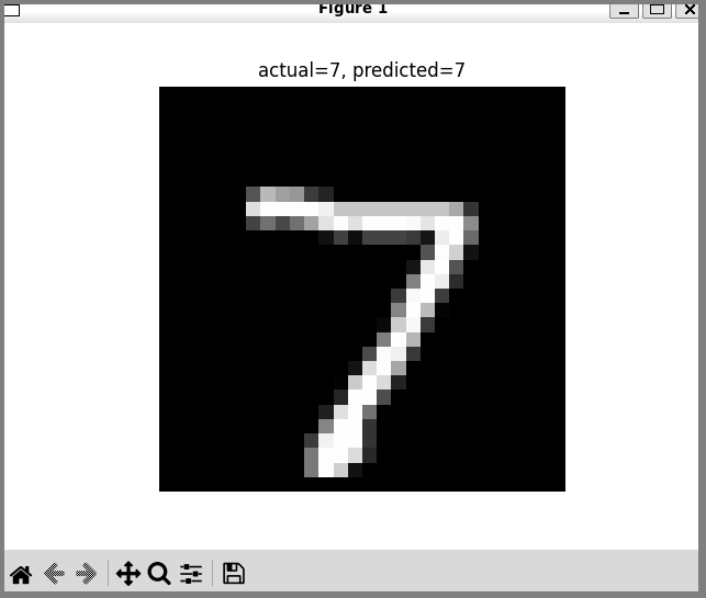
plt.imshow(X_sample.squeeze(), cmap="gray")
plt.title(f"actual={Y_sample}, predicted={pred}")
plt.axis("off")
plt.show()
4.2 d4_api_mnist.py
# d4_api_mnist.py
import torch
import torch.nn as nn
import torch.nn.functional as F

from fastapi import FastAPI
from pydantic import BaseModel


app = FastAPI()

device = "cpu"


class DigitPixels(BaseModel):
    pixels: list[list[float]]  # 28 rows x 28 columns


class TinyCNN(nn.Module):
    def __init__(self):
        super().__init__()

        self.conv1 = nn.Conv2d(1, 8, kernel_size=3, padding=1)
        self.conv2 = nn.Conv2d(8, 16, kernel_size=3, padding=1)

        self.pool = nn.MaxPool2d(2, 2)

        self.fc1 = nn.Linear(16 * 7 * 7, 64)
        self.fc2 = nn.Linear(64, 10)

    def forward(self, x):
        x = self.pool(F.relu(self.conv1(x)))  # [batch, 8, 14, 14]
        x = self.pool(F.relu(self.conv2(x)))  # [batch, 16, 7, 7]

        x = x.reshape(x.size(0), -1)          # [batch, 784]

        x = F.relu(self.fc1(x))               # [batch, 64]
        x = self.fc2(x)                       # [batch, 10]

        return x


model = TinyCNN().to(device)

model.load_state_dict(
    torch.load("d4_cnn.pt", map_location=device)
)

model.eval()


@app.get("/")
def root():
    return {
        "ok": True,
        "demo": "D4 MNIST CNN API",
        "endpoint": "POST /predict",
    }


@app.post("/predict")
def predict(data: DigitPixels):
    X = torch.tensor(data.pixels, dtype=torch.float32)

    # expected shape: [28, 28]
    if X.shape != (28, 28):
        return {
            "error": "pixels must be a 28x28 array"
        }

    # convert to CNN input shape: [batch, channel, height, width]
    X = X.unsqueeze(0).unsqueeze(0).to(device)

    with torch.no_grad():
        logits = model(X)
        pred = logits.argmax(dim=1).item()
        probs = torch.softmax(logits, dim=1)[0]

    return {
        "predicted_digit": pred,
        "confidence": float(probs[pred]),
        "probabilities": [float(p) for p in probs],
    }
4.3 d4_test_api.py
# d4_test_api.py

import requests
from torchvision import datasets, transforms

test_data = datasets.MNIST(
    root="data",
    train=False,
    download=True,
    transform=transforms.ToTensor(),
)

X, Y = test_data[0]

payload = {
    "pixels": X.squeeze().tolist()
}

r = requests.post(
##    "http://127.0.0.1:8000/predict",
    "https://six07-core-nns-d4.onrender.com/predict",
    json=payload,
)

print("actual:", Y)
print(r.json())
3.1.2b Tiny CNN (D4)
See 2.2.1 D4 CNN image classifier and (for details) 2.2.1b D4 CNN algorithm details.
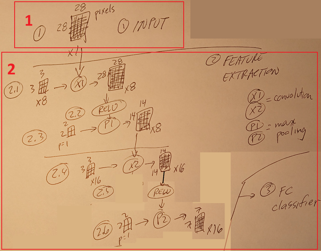
There are 3 main parts.
- 1 Data input. In this case the data input is ………….
- 2 Feature extraction (nn.Conv2d + nn.MaxPool2d). This is where convolution and pooling are used to turn the original pixel values into “hidden state” values that progressive define higher level features (I typical call these values “pix’s”). …
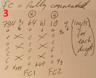
- 3 Final NN (nn.Linear) computing CNN “logits”. This involves
- 3.1 Linear NN (like for D2ccc) computes the probabilities of each of 10 possible outputs (digits 0 to 9).
- 3.2 The most probable output is converted into a label (such as “7”).
class TinyCNN(nn.Module):
    def __init__(self):
        super().__init__()
        self.conv1 = nn.Conv2d(1, 8, kernel_size=3, padding=1)
        self.conv2 = nn.Conv2d(8, 16, kernel_size=3, padding=1)
        self.pool = nn.MaxPool2d(2, 2)
        self.fc1 = nn.Linear(16 * 7 * 7, 64)
        self.fc2 = nn.Linear(64, 10)
26.0616 (0527)